The ezPurrr package is built on top of the purrr library. The purpose of the package is to help make functional programming workflows more simple and efficient. Let’s start by loading ezPurrr and a few other packages we’ll use for data manipulation in this vignette.
ezPurrr requires a nested dataset. For example
nest_df <- palmerpenguins::penguins %>%
  group_by(island, species) %>%
  nest()

head(nest_df)
#> # A tibble: 5 × 3
#> # Groups:   island, species [5]
#>   species   island    data
#>   <fct>     <fct>     <list>
#> 1 Adelie    Torgersen <tibble [52 × 6]>
#> 2 Adelie    Biscoe    <tibble [44 × 6]>
#> 3 Adelie    Dream     <tibble [56 × 6]>
#> 4 Gentoo    Biscoe    <tibble [124 × 6]>
#> 5 Chinstrap Dream     <tibble [68 × 6]>
This data frame has columns for the penguin species and the island on which the data was collected but, critically, an additional data column. This column is a list column that has all the data for the corresponding species/island row. All functions in ezPurrr require the data to first be in this format.
From here, we want to be able to work with the data like normal, but it’s difficult when the data are in this list column format. This is where teh sample_*() functions come in.
sample_*()
sample_row()
The sample_row() function returns one random or one particular row (when an index argument is supplied) from the nested data as a list or a data frame. If returning a list (default), the first item of the list with be the data from the given row, while the remaining elements of the list will be the grouping variables from that row (i.e., the species and island for the corresponding row, in our previous example). If returning a data frame (with type = df argument), then the data frame will include one row of the nested data, as well as each grouping variable as a column (with identical repeated content).
For example
nest_df %>%
  sample_row()
#> row 5 is selected randomly
#> $data
#> # A tibble: 68 × 6
#>    bill_length_mm bill_depth_mm flipper_length_mm body_mass_g sex     year
#>             <dbl>         <dbl>             <int>       <int> <fct>  <int>
#>  1           46.5          17.9               192        3500 female  2007
#>  2           50            19.5               196        3900 male    2007
#>  3           51.3          19.2               193        3650 male    2007
#>  4           45.4          18.7               188        3525 female  2007
#>  5           52.7          19.8               197        3725 male    2007
#>  6           45.2          17.8               198        3950 female  2007
#>  7           46.1          18.2               178        3250 female  2007
#>  8           51.3          18.2               197        3750 male    2007
#>  9           46            18.9               195        4150 female  2007
#> 10           51.3          19.9               198        3700 male    2007
#> # … with 58 more rows
#>
#> $island
#> [1] Dream
#> Levels: Biscoe Dream Torgersen
#>
#> $species
#> [1] Chinstrap
#> Levels: Adelie Chinstrap Gentoo

nest_df %>%
  sample_row(index = 3) %>%
  head()
#> $data
#> # A tibble: 56 × 6
#>    bill_length_mm bill_depth_mm flipper_length_mm body_mass_g sex     year
#>             <dbl>         <dbl>             <int>       <int> <fct>  <int>
#>  1           39.5          16.7               178        3250 female  2007
#>  2           37.2          18.1               178        3900 male    2007
#>  3           39.5          17.8               188        3300 female  2007
#>  4           40.9          18.9               184        3900 male    2007
#>  5           36.4          17                 195        3325 female  2007
#>  6           39.2          21.1               196        4150 male    2007
#>  7           38.8          20                 190        3950 male    2007
#>  8           42.2          18.5               180        3550 female  2007
#>  9           37.6          19.3               181        3300 female  2007
#> 10           39.8          19.1               184        4650 male    2007
#> # … with 46 more rows
#>
#> $island
#> [1] Dream
#> Levels: Biscoe Dream Torgersen
#>
#> $species
#> [1] Adelie
#> Levels: Adelie Chinstrap Gentoo

nest_df %>%
  sample_row(index = 3, type = 'df') %>%
  head()
#> # A tibble: 6 × 8
#>   bill_length_mm bill_depth_mm flipper_length_mm body_mass_g sex     year
#>            <dbl>         <dbl>             <int>       <int> <fct>  <int>
#> 1           39.5          16.7               178        3250 female  2007
#> 2           37.2          18.1               178        3900 male    2007
#> 3           39.5          17.8               188        3300 female  2007
#> 4           40.9          18.9               184        3900 male    2007
#> 5           36.4          17                 195        3325 female  2007
#> 6           39.2          21.1               196        4150 male    2007
#> # … with 2 more variables: group.island <fct>, group.species <fct>
sample_data()
sample_data() returns one random or one particular data column (with index argument) from the nested data. The primary difference between sample_data() versus sample_row() is that the grouping variables are not returned - just the data. For example:
nest_df %>%
  sample_data()
#> row 2 is selected randomly
#> # A tibble: 44 × 6
#>    bill_length_mm bill_depth_mm flipper_length_mm body_mass_g sex     year
#>             <dbl>         <dbl>             <int>       <int> <fct>  <int>
#>  1           37.8          18.3               174        3400 female  2007
#>  2           37.7          18.7               180        3600 male    2007
#>  3           35.9          19.2               189        3800 female  2007
#>  4           38.2          18.1               185        3950 male    2007
#>  5           38.8          17.2               180        3800 male    2007
#>  6           35.3          18.9               187        3800 female  2007
#>  7           40.6          18.6               183        3550 male    2007
#>  8           40.5          17.9               187        3200 female  2007
#>  9           37.9          18.6               172        3150 female  2007
#> 10           40.5          18.9               180        3950 male    2007
#> # … with 34 more rows

nest_df %>%
  sample_data(index = 3)
#> # A tibble: 56 × 6
#>    bill_length_mm bill_depth_mm flipper_length_mm body_mass_g sex     year
#>             <dbl>         <dbl>             <int>       <int> <fct>  <int>
#>  1           39.5          16.7               178        3250 female  2007
#>  2           37.2          18.1               178        3900 male    2007
#>  3           39.5          17.8               188        3300 female  2007
#>  4           40.9          18.9               184        3900 male    2007
#>  5           36.4          17                 195        3325 female  2007
#>  6           39.2          21.1               196        4150 male    2007
#>  7           38.8          20                 190        3950 male    2007
#>  8           42.2          18.5               180        3550 female  2007
#>  9           37.6          19.3               181        3300 female  2007
#> 10           39.8          19.1               184        4650 male    2007
#> # … with 46 more rows
sample_group()
Finally, sample_group() returns one random or one particular grouping columns (with index argument) from the nested dataset with no data. For example:
nest_df %>%
  sample_group()
#> row 3 is selected randomly
#> # A tibble: 1 × 2
#> # Groups:   island, species [1]
#>   species island
#>   <fct>   <fct>
#> 1 Adelie  Dream

nest_df %>%
  sample_group(index = 3)
#> # A tibble: 1 × 2
#> # Groups:   island, species [1]
#>   species island
#>   <fct>   <fct>
#> 1 Adelie  Dream
broadcast()
broadcast()
Generally, we will use the data we have sampled to conduct some operations. Once we’ve conducted those operations we just need to wrap them all in a function, then broadcast() them across the sets of data (i.e., all rows).
In other words, the sampling dataset is used to test the code you want to be applied for each row, such as figures, models, or transformations.
Let’s look at an example for plotting. First, we create our sample data.
samp <- nest_df %>%
  sample_data(index = 3)

samp
#> # A tibble: 56 × 6
#>    bill_length_mm bill_depth_mm flipper_length_mm body_mass_g sex     year
#>             <dbl>         <dbl>             <int>       <int> <fct>  <int>
#>  1           39.5          16.7               178        3250 female  2007
#>  2           37.2          18.1               178        3900 male    2007
#>  3           39.5          17.8               188        3300 female  2007
#>  4           40.9          18.9               184        3900 male    2007
#>  5           36.4          17                 195        3325 female  2007
#>  6           39.2          21.1               196        4150 male    2007
#>  7           38.8          20                 190        3950 male    2007
#>  8           42.2          18.5               180        3550 female  2007
#>  9           37.6          19.3               181        3300 female  2007
#> 10           39.8          19.1               184        4650 male    2007
#> # … with 46 more rows
Next, we write the code to create our plot, using samp as our sample data to test our code.
ggplot(samp, aes(x = bill_length_mm,
                 y = bill_depth_mm,
                 color = body_mass_g)) +
  geom_point()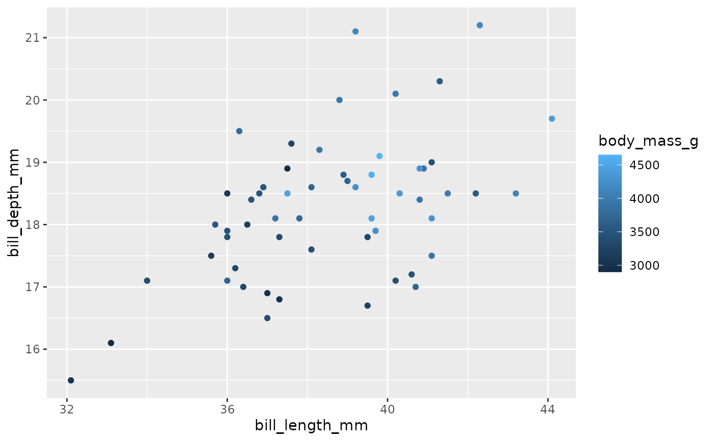
Finally, we can wrap this into a function.
plotting <- function(data){
  ggplot(data, aes(x = bill_length_mm,
                   y = bill_depth_mm,
                   color = body_mass_g)) +
    geom_point()
}
Notice the code above is exactly as we had before, we’ve just changed our sample data set to data as an argument within a function. Normally, writing functions for plotting (and many other functions in the tidyverse) is difficult because of non-standard evaluation, but in this case we don’t have to worry about any of that.
Now, we can broadcast() the function to all of the data!
broadcasted_df = nest_df %>%
  broadcast(plotting)
broadcasted_df
#> # A tibble: 5 × 4
#> # Groups:   island, species [5]
#>   species   island    data               output
#>   <fct>     <fct>     <list>             <list>
#> 1 Adelie    Torgersen <tibble [52 × 6]>  <gg>
#> 2 Adelie    Biscoe    <tibble [44 × 6]>  <gg>
#> 3 Adelie    Dream     <tibble [56 × 6]>  <gg>
#> 4 Gentoo    Biscoe    <tibble [124 × 6]> <gg>
#> 5 Chinstrap Dream     <tibble [68 × 6]>  <gg>
Notice we now have a new column, called output, which has all the plots! To look at the first plot, we can print it with
broadcasted_df$output[[1]]
#> Warning: Removed 1 rows containing missing values (geom_point).
Or, similarly:
broadcasted_df %>%
  pull(output) %>%
  purrr::pluck(1)
#> Warning: Removed 1 rows containing missing values (geom_point).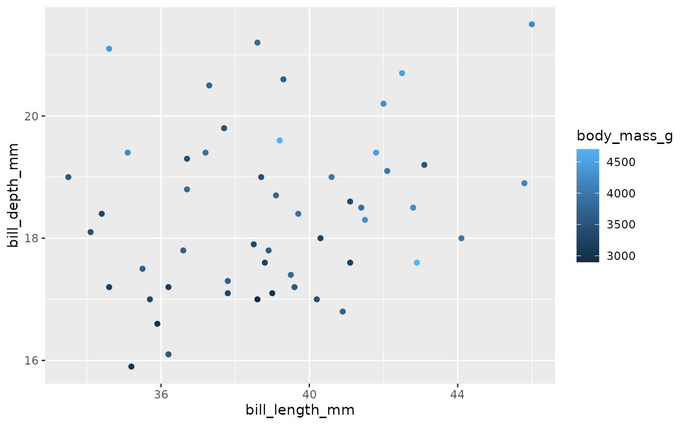
You can also use it for modeling or other functions. For example:
tmp_df = nest_df %>%
  sample_data(index = 3)

lm(body_mass_g ~ bill_length_mm * bill_depth_mm, data = tmp_df)
#>
#> Call:
#> lm(formula = body_mass_g ~ bill_length_mm * bill_depth_mm, data = tmp_df)
#>
#> Coefficients:
#>                  (Intercept)                bill_length_mm
#>                   -2079.0346                       92.6987
#>                bill_depth_mm  bill_length_mm:bill_depth_mm
#>                     145.9699                       -0.6616

modeling <- function(data){
   lm(body_mass_g ~ bill_length_mm + bill_depth_mm, data = data)
}

nest_df %>%
  broadcast(modeling) %>%
  .$output
#> [[1]]
#>
#> Call:
#> lm(formula = body_mass_g ~ bill_length_mm + bill_depth_mm, data = data)
#>
#> Coefficients:
#>    (Intercept)  bill_length_mm   bill_depth_mm
#>       -1161.63           47.79          163.14
#>
#>
#> [[2]]
#>
#> Call:
#> lm(formula = body_mass_g ~ bill_length_mm + bill_depth_mm, data = data)
#>
#> Coefficients:
#>    (Intercept)  bill_length_mm   bill_depth_mm
#>       -3015.76           86.27          183.06
#>
#>
#> [[3]]
#>
#> Call:
#> lm(formula = body_mass_g ~ bill_length_mm + bill_depth_mm, data = data)
#>
#> Coefficients:
#>    (Intercept)  bill_length_mm   bill_depth_mm
#>       -1622.93           80.87          120.41
#>
#>
#> [[4]]
#>
#> Call:
#> lm(formula = body_mass_g ~ bill_length_mm + bill_depth_mm, data = data)
#>
#> Coefficients:
#>    (Intercept)  bill_length_mm   bill_depth_mm
#>       -1452.12           57.64          252.96
#>
#>
#> [[5]]
#>
#> Call:
#> lm(formula = body_mass_g ~ bill_length_mm + bill_depth_mm, data = data)
#>
#> Coefficients:
#>    (Intercept)  bill_length_mm   bill_depth_mm
#>        -356.11           23.82          158.84
Instead of a list, you can also make the output a number (double).
modeling <- function(data){
  model = lm(body_mass_g ~ bill_length_mm + bill_depth_mm, data = data)
  model$coefficients[2] # the slope for bill_length_mm
}

nest_df %>% broadcast(modeling) %>% .$output
#> [[1]]
#> bill_length_mm
#>       47.78764
#>
#> [[2]]
#> bill_length_mm
#>       86.27406
#>
#> [[3]]
#> bill_length_mm
#>       80.86942
#>
#> [[4]]
#> bill_length_mm
#>       57.64173
#>
#> [[5]]
#> bill_length_mm
#>       23.82257
broadcast_group()
broadcast_group() allows you to also use grouping variables in the function. It is still under development so currently it only works in a more limited way. For example, you can include grouping variables as the title for plots.
df = nest_df %>%
  sample_row(index = 3, type = 'list')

plotting = function(data, species, island){
  ggplot(data, aes(x = bill_length_mm,
                             y = bill_depth_mm,
                             color = body_mass_g)) +
    geom_point() +
    labs(title = paste(species, island))
}

# example with a single plot
plotting(df$data, df$species, df$island)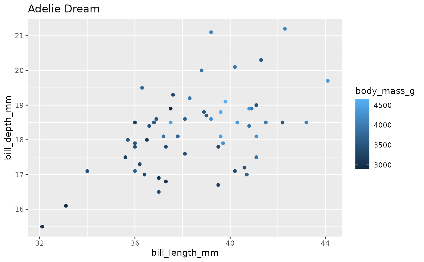
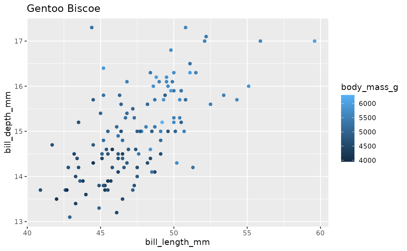
nest_df = nest_df %>%
  broadcast_group(plotting)

nest_df$output[[1]]
#> Warning: Removed 1 rows containing missing values (geom_point).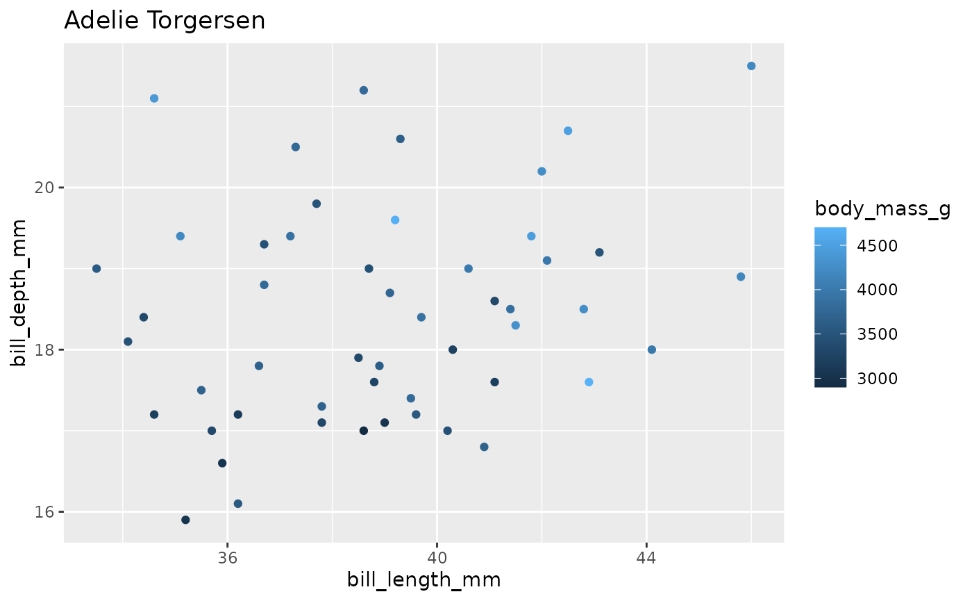
nest_df$output[[4]]
#> Warning: Removed 1 rows containing missing values (geom_point).